Experts have designed these Class 9 Maths Notes and Chapter 2 Introduction to Linear Polynomials Class 9 Ganita Manjari Notes for effective learning.
Class 9 Maths Chapter 2 Introduction to Linear Polynomials Notes
Class 9 Maths Ganita Manjari Chapter 2 Notes
Ganita Manjari Class 9 Chapter 2 Notes – Class 9 Introduction to Linear Polynomials Note
In this chapter, we will introduce algebraic expressions and polynomials and learn to identify their terms, coefficients and degree. We will explore linear polynomials and relationship, including slope and y-intercept and represent them using equations and graphs.
The chapter also connects algebra to real-life situations through linear growth and pattern analysis.
Introduction to Polynomials
Variables usually denoted by the letters x, y, z etc. They can take various numerical values. Constants have a fixed numerical value throughout a particular solution, e.g. -4, 3, π etc.
Algebraic Expressions
A combination of constants and variables, connected by the four fundamental arithmetical operations +, x and 4- is called an algebraic expression.
e.g. 6x2 – 5y2 +2xy is an algebraic expression, where xandy are variables and 6, -5, 2 are constants.
An algebraic expression in which the variables involved only non-negative integral power, is called a polynomial, e.g. x2 – 3xy – 7y + 2
Polynomials
A polynomials in one variable x, is an algebraic expression of the form
anxn + an-1xn-1 + an-2xn-2 +… + a2x2 + a1x + a0 = p(x) [say]
where, n is a non-negative integer and a0,a1,a2,…,an are constants (real numbers).
The constants a0, a1, a2,.., an are also known as coefficients of polynomials.
Example 1:
Which of the following are polynomials? Justify your answer.
(i) x3 + 3x2 + 2
(ii) \(\sqrt{x^5}\) + 4x + 2
(iii) \(\frac{x^4+x^3+3 x^2+2 x}{x^2}\)
Solution:
(i) Given expression is x3 + 3x2 + 2.
Here, we see that the variable x has all non-negative integer powers.
Hence, it is a polynomial.
(ii) Given expression is \(\sqrt{x^5}\) + 4x + 2 or x5/2 + 4x + 2.
Here, we see that the variable x does not have all non-negative integer powers.
Clearly, \(\sqrt{x^5}\) i.e. x5/2 does not have a non-negative integer power.
Hence, it is not a polynomial.
(iii) Given expression is
\(\frac{x^4+x^3+3 x^2+2 x}{x^2}\) or x2 + x + 3 + \(\frac{2}{3}\)
Here, we see that the variable x does not have all non-negative integer powers.
Hence, it is not a polynomial.
Example 2:
Which of the following expressions are polynomials in one or more variable(s)? State reasons for your answer.
(i) 3x2 – 5x
(ii) 5y2 + 8x
(iii) √t + 3y
(iv) x3 + x2 + \(\frac{1}{x}\)
Solution:
(i) Given expression is 3x2 – 5x.
Here, expression is in one variable and all powers of the variable are non-negative integers.
Hence, it is a polynomial in one variable.
(ii) Given expression is 5y2 + 8x.
Here, expression is in two variables and all powers of variables are non-negative integers.
Hence, it is a polynomial in two variables.
(iii) Given expression is √t + 3y or t1/2 + 3y and all powers of variables are not non-negative integers. Hence, it is not a polynomial.
(iv) Given expression is x3 + x2 + \(\frac{1}{x}\) or x3 + x2 + x-1.
Here, the expression is in one variable and all powers of the variable are not non-negative integers.
Hence, it is not a polynomial.
Term and Coefficient of a Polynomial
The part of a polynomial separated by V or sign is called a term of the polynomial. Each term of a polynomial has a coefficient, which is the constant associated with that term.
e.g. In polynomial x2 – 4x + 7, the expressions x2, 4x and 7 are called terms of the polynomial and here coefficient of x2 is 1, coefficient of x is -4 and coefficient of x° i.e. constant term is 7.
Example 3:
Find the coefficient of x2 in (3x + x3)(x + \(\frac{1}{x}\))
Solution:
We have, (3x + x3)(x + \(\frac{1}{x}\))
= 3x × x + 3x × (x + \(\frac{1}{x}\)) + x3 × x + x3 × \(\frac{1}{x}\)
= 3x2 + 3 + x4 + x2
= x4 + 4x2 +3
So, the coefficient of x2 is 4.
Degree of a Polynomial
Highest power of the variable in a polynomial is known as the degree of polynomial.
![]()
Example 4:
Find the degree of the following polynomials.
(i) 2x4 – 6x3 + 4x + 1
Solution:
We have, 2x4 – 6x3 + 4x + 1
Here, the highest power of x is 4, so its degree is 4.
(ii) \(\frac{1}{2}\)x – 5x2 + \(\frac{1}{2}\)x3 + x5
Solution:
We have, \(\frac{1}{2}\)x – 5x2 + \(\frac{1}{2}\)x3 + x5
Here, the highest power of x is 5, so its degree is 5.
(iii) 6x + √3
Solution:
We have, 6x + √3
Here, the highest power of x is 1, so its degree is 1.
(iv) 7x2 + 2x + 5
Solution:
We have, 7x2 + 2x + 5
Here, the highest power of x is 2, so its degree is 2.
(v) 4
Solution:
We have, 4 i.e. 4 x°.
Here, the exponent of x is 0, so its degree is 0.
Classifications of Polynomials
On the Basis of Number of Terms
(i) Monomial A polynomial containing one non-zero term is called a monomial (‘mono’ means ‘one’), e.g. 5x, 7, 3x3, -7x2 and u4 are monomials.
(ii) Binomial A polynomial containing two non-zero terms, is called a binomial (‘bi’ means ‘two’).
e.g. 5 +7x, 7x2y + 3y, y30 +1 and z23 – z2 are binomials.
(iii) Trinomial A polynomial containing three non-zero terms is called a trinomial (‘tri’ means ‘three’).
e.g. 8 + 3x + x2, 7 + 5xy + 6xy2 and √2 + x – x2 are trinomials.
Example 5:
Identify the types of polynomials on the basis of terms from the following.
(i) 4y + 3y2 + 6
Solution:
We have, 4y + 3y2 + 6
Here, number of terms in given polynomial is 3. Hence, it is a trinomial.
(ii) 3x + 2
Solution:
We have, 3x + 2
Here, number of terms in given polynomial is 2. Hence, it is a binomial.
(iii) 6t
Solution:
We have, 6t
Here, number of terms in given polynomial is 1. Hence, it is a monomial.
On the Basis of Degree of Variables
(i) Constant Polynomial A polynomial of degree zero, is called constant polynomial.
Or
A polynomial containing only one constant term is called a constant polynomial.
e.g. 3, -7 and \(\frac{7}{4}\) are constant polynomials.
(ii) Linear Polynomial A polynomial of degree 1, is called a linear polynomial.
e.g. 2x + 5 is a linear polynomial in x.
Thus, we observe that a linear polynomial in x will have atmost two terms.
So, standard form of a linear polynomial in x will be ax +b, where a and b are constants and a + 0.
(iii) Quadratic Polynomial A polynomial of degree 2 is called a quadratic polynomial.
e.g. 3x2 + 7x + 9 is a quadratic polynomial in x.
Thus, we observe that a quadratic polynomial in x will have atmost 3 terms.
So, a quadratic polynomial in x is of the form ax2 + bx + c, where a, b and c are constants and a ∈ 0.
(iv) Cubic Polynomial A polynomial of degree 3 is called a cubic polynomial.
e.g. 6y3 +7y2 – 5y + 1 is a cubic polynomial in y.
Thus, we observe that a cubic polynomial in y will have atmost 4 terms.
So, a cubic polynomial in x is of the form ax3 + bx2 + cx + d, where a,b, c and d are constants and a + 0.
(vi) n Degree Polynomial A polynomial of degree n in x is an expression of the form
p(x) = anxn + an-1xn-1 + an-2xn-2 + ……… + a2x2 + a1x + a0
where, an, an-1 …. a2, a1, a0 are constants and an ≠ 0.
Here, anxn, an-1xn-1, an-2xn-2, ……… , a2x2, a1x, a0 are known as the terms of the polynomial p(x) and an, an-1 …. a2, a1, a0 are known as their coefficients.
(vii) Zero Polynomial If a0 = a1 = a2 = … = an = 0 (all constants are zero) then we get the zero polynomial, which is denoted by 0.
If p(x) = 0 then it is called the zero polynomial. But, the degree of zero polynomial is not defined as p(x) can be written as p(x) = 0 = 0. x = 0. x2 = 0. x3 = …
The zero polynomial is also known as constant polynomial.
Example 6.
Identify the types of polynomials, on the basis of degree from the following.
(i) 3x2 +5
(ii) z3 + 4z + 1
(iii) 4t
Solution:
(i) We have, 3x2 + 5
Here, degree of polynomial 3x2 + 5 is 2.
Hence, it is a quadratic polynomial.
(ii) We have, z3 + 4z +1
Here, degree of polynomial z3 + 4z + 1 is 3.
Hence, it is a cubic polynomial.
(iii) We have, 4t
Here, degree of polynomial 4t is 1.
Hence, it is a linear polynomial.
Example 7.
Give an example of polynomial, which is
(i) monomial of degree 3?
(ii) binomial of degree 15?
(iii) trinomial of degree 7?
Solution:
(i) 2x3
(ii) x15 + 12x
(iii) y7 + y5 + y3
Example 8.
Write each of the following equations in the form ax + by + c=0 and indicate the values of a, band c in each case.
(i) 3x – 5y = 7.82
(ii) y – 6 = √5x
(iii) 8 = 2x + 9y
(iv) 4x = -7y
Solution:
(i) 3x – 5y = 7.82 ⇒ 3x – 5y – 7.82 = 0
On comparing with ax + by + c = 0, we get a = 3, b = -5 and c = -7.82
(ii) 7 – 6 = -√5x ⇒ – √5x + 7 – 6 = 0
On comparing with ax + by + c = 0, we get a = -√5, b = 1 and c = -6
(iii) 8 = 2x + 97 ⇒ -2x – 97 + 8 = 0
On comparing with ax + by + c = 0, we get a = -2, b – 9 and c = 8
(iv) 4x = -7y ⇒ 4x + 7y = 0
On comparing with ax + by + c = 0, we get a = 4, b = 7 and c = 0
Example 9.
Write each of the following as an equation in two variables
(i) 2x = -9
(ii) 5y = 3
(iii) x = 0
Solution:
(i) 2x = -9 can be written as 2 – x + 0 – 7 + 9 = 0
(ii) 57 = 3 can be written as 0 – x + 5 – 7 – 3 = 0
(iii) x = 0 can be written as 1 – x + 0 – 7 + 0 = 0
Example 10.
For what value of m, the expression
x(m2 – 1) + 5x\(\frac{m}{2}\) will be a cubic polynomial?
Solution:
Given expression is x(m2 – 1) + 5x\(\frac{m}{2}\)
For it to be a cubic polynomial, the highest power of x must be 3.
Here, the powers of x are m2 – 1 and \(\frac{m}{2}\).
Case I: If m2 – 1 = 3 => m2 = 4
⇒ m = ± 2
When m = -2, \(\frac{m}{2}=\frac{-2}{2}\) = -1
Since, the power -1 is not a non-negative integer, so the expression is not a polynomial for m = -2.
Thus, m = 2
Case II: If – =3 ⇒ m = 6
Then, m2 – 1 = (6)2 – 1 = 35
Then, the highest power would be 35, not 3.
So, m = 6 is not a solution.
Hence, m = 2 is the only value for which the given expression will be a cubic polynomial.
![]()
Application of Linear Polynominals and Linear Patterns
Value of a Polynomial
The number obtained by substituting a particular value of the variable in a polynomial is called the value of the polynomial at that point. The value of a polynomial p(x) at x =a (say) is denoted by p(a).
Example .
Find the value of each of the following polynomials at the indicated value of variables.
(i) p(x) = 5x3 – 2x2 + 3x – 2 at x = 1.
Solution:
We have, p(x) = 5x3 – 2x2 + 3x – 2
On putting x = 1 in p (x), we get p( 1) = 5(1)3 – 2(1)2 + 3(1) – 2
= 5 – 2 + 3 – 2
= 8 – 4
= 4, which is the required value of p (x) at x = 1.
(ii) q(y) = 3y3 – 4y + \(\sqrt{11}\) at y = 2.
Solution:
We have, q(y) = 3y3 – 4y + \(\sqrt{11}\)
On putting y = 2 in q(y), we get
q(2) = 3(2)3 – 4(2) + \(\sqrt{11}\)
= 3 × 8 – 8 + \(\sqrt{11}\)
= 24 – 8 + \(\sqrt{11}\)
= 16 + \(\sqrt{11}\) ,
which is the required value of q(y) at y = 2.
(iii) p(t) = 4t4 + 5t3 – t2 + 6 at t = a.
Solution:
We have,p(f) = 4t4 + 5t3 – t2 + 6
On putting t = a in p (t), we get
p(a) = 4(a)4 + 5(a)3 – (a)2 +6
= 4a4 + 5a3 – a2 + 6, which is the required value of p(t) at t = a.
Application of Linear Polynomial
A polynomial of degree 1 is called a linear polynomial.
For instance, ax + by + c (where, a ≠ 0 and b ≠ 0) is a linear polynomial. The primary application of linear polynomials is obtaining equations to represent and solve for unknown quantities in real-life situations.
A statement of equality involving one or more variables is called an equation. When we equate a linear polynomial to zero, we obtain a linear equation i.e. linear equation ax + by + c = 0 (where, a ≠ 0, b ≠ 0).
e.g. Since, the runs scored by two cricket players are unknown, there are two unknown quantities or variables. Let the runs scored by Rahul be x and by Simran be y. If they built a total partnership of 150 runs in a match, the required equation is x + y = 150.
This is an example of a linear equation in two variables. We can write this in the standard form as x + y – 150 = 0.
Example 2.
The present age of Ravi’s father is four times Ravi’s present age. After 6 yr, their ages will add upto 72 yr. Find their present ages.
Solution:
Let the present age of Ravi be x yr.
Therefore, the present age of Ravi’s father is 4xyr.
According to the question,
(x + 6) + (4x + 6) = 72
⇒ x + 6 + 4x + 6 = 72
⇒ 5x + 12 = 72
⇒ 5x = 72 – 12
⇒ 5x = 60
Thus, Ravi’s present age, x = 12 yr.
Therefore, Ravi’s father’s present age, 4x = 4 × 12 = 48 yr.
Example 3.
The difference between two positive integers is 48. The ratio of the two integers is 3 : 7. Find the two integers.
Solution:
Let the two integers be 3x and 7x, where x is a common factor.
According to the question,
7x – 3x = 48
⇒ 4x = 48
⇒ x = \(\frac{48}{4}\) = 12
3x = 3 × 12 = 36
and 7x =7 × 12 =84
Hence, the two integers are 36 and 84.
Exploring Linear Patterns
When a sequence of numbers or a table of values shows that the value of y changes by a constant amount every time x increases by 1, it forms a linear pattern. In algebra such patterns can always be represented by a linear polynomial of the form ax +b.
e.g. Observe the following table.
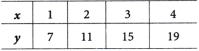
When x = 1, y = 7 = 4 × 1 + 3
When x = 2, y = 11 = 4 × 2 + 3 [11 – 7 = 4]
When x = 3, y = 15 = 4 × 3 + 3 [15 – 11 = 4]
The value of y increases by 4.
So, the linear polynomial for this pattern is p(x) = 4x + 3. Hence, a linear pattern is a sequence of numbers or figures in which the change between consecutive terms is constant.
Or
When a pattern increases or decreases by the same amount each step, it is called a linear pattern.
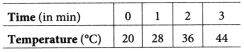
Example 4:
The temperature of a heated liquid over time is given in the table. Find whether the pattern is linear or not.
Solution:
Let’s observe the change in temperature for each consecutive minute.
Change in 1 st min ⇒ 28 – 20 = 8
Change in 2nd min ⇒ 36 – 28 = 8
Change in 3rd min ⇒ 44 – 36 = 8
Here, the temperature increases by a constant amount of 8°C every minute. Hence, the pattern is linear.
Example 5.
A girl has ₹ 400 saved in her bank account. She receives ₹ 120 every month as allowance. Determine the amount she will have at the end of each month starting from the second month. Also, form a linear expression for the total amount after n months.
Solution:
Given, initial amount (c) = ₹ 400
and rate of change (m) = + 120 per month
Now, linear expression y = 120n + 400
Where, y is the total amount and n is the number of months. To find how much money she will have from the second month onwards, we substitute the values of n .
At the end of the 2nd month (n = 2),
y = 120(2) + 400 = 240 + 400 = ₹ 640
At the end of the 3rd month (n = 3),
y = 120(3) + 400 = 360 + 400 = ₹ 760
At the end of the 4th month (n = 4),
y = 120(4) + 400 = 480 + 400 = ₹ 880
![]()
Example 6.
A rectangular box has length 6 cm and breadth 9 cm. Calculate the volume, when the height is
(i) 4 cm
(ii) 8 cm
(ii) 12 cm.
Also, obtain the linear expression showing the relation between volume and height.
Solution:
Given, length (l) = 6 cm and breadth (b) = 9 cm.
Now, volume of rectangular box,
y = l × b × h
⇒ y = 6 × 9 × h
⇒ y = 54h
Where, y is the volume and h is the height.
(i) For h = 4,
y = 54(4) = 216 cm3
(ii) For h = 8,
y = 54(8) = 432 cm3
(ii) For h = 12,
y = 54(12) = 648 cm3
Example 7.
Riya is reading a book of 480 pages. She reads 16 pages every day. How many pages will be left after 15 days? Express this as a linear pattern.
Solution:
Given, total pages (c) = 480
and rate of change (m) = -16 pages per day
Now, polynomial expression,
y = – 16x + 480
Where, y is the remaining pages and x is the number of days.
After 15 days (x = 15), the remaining pages are y = -16(15) + 480 = -240 + 480 = 240
Thus, the pages left after 15 days are 240.
Visualising Linear Relationship and Graph of Linear Equation in Two Variables
Visualising Linear Relationships
In algebra, a linear polynomial in two variables is of the form ax + by +c -0, where a, b and c are constants and a, b are not both zero. Such an equation represents a linear relationship between x andy.
To visualise a linear relationship means to represent all the solutions of a linear equation graphically on the coordinate plane, each solution (x, y) is taken as an ordered pair and plotted as a point. When all such points are plotted, they lie on a straight line.
Thus, a linear polynomial in two variables always represents a straight line, when graphed.
Graph of a Linear Equation in Two Variables
We know that a linear equation ax+by+c-0 in two variables x and y has infinitely many solutions.
If we plot these solutions on a graph paper, we see that each solution represents a point and on joining these points, we get a straight line, such a straight line is called the graph of the linear equation.
Thus, we can conclude that every point on the line satisfies the equation of the line i.e. every point on the line is a solution of the equation and every solution of the equation is a point on the line.
Method to Draw The Graph of Linear Equation in Two Variables
Let the linear equation in two variables be ax + by + c = 0, where a ≠ 0, b ≠ 0 and x, y are variables. Then, to draw its graph, we use the following steps.
Step I
Write given linear equation and express y in terms of x
i. e. by = -(ax + c) ⇒ y = \(-\frac{(a x+c)}{b}\) …(1)
Step II
Put different arbitrary values of x in Eq.(i) and find the corresponding values of y.
Step III
Form a table as follows, by writing the values of y below the corresponding values of x.
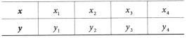
Step IV
Draw the coordinate axes on graph paper and take a suitable scale to plot points (x1, y1), (x2, y2),… on graph paper.
Step V
Join these points (x1, y1), (x2, y2),… . Thus, we get a straight line and produce it on both sides.
Hence, the straight line, so obtained is the required graph of given linear equation. Similarly, we can draw the graph of more than one linear equation in two variables.
Note:
- If possible, choose the integral values of x in Step II in such a way that the corresponding values of y are also integers.
- It is enough to plot two points corresponding to two solutions and join them by a line. However, it is advisable to plot more than two such points so that the correctness of the graph may be checked immediately.
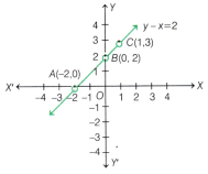
Example 1:
Draw the graph of the equation y – x =2.
Solution:
Given, linear equation can be written as y = 2 + x …(i)
When, x = -2 then from Eq. (i), we get y = 2 – 2 = 0
When, x = 0 then from Eq. (i), we get y = 2
When, x = 1 then from Eq. (i), we get y = 2 + 1 = 3
Thus, we get the table
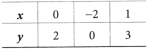
Draw the coordinate axesXOX’ and TO X and plot the points A(-2, 0 ),B (0, 2) and C(1, 3) by taking a suitable scale.
On joining the points A, B and C, we get a straight line AC. Thus, the line AC represents the required graph of given linear equation in two variables.
Note:
An equation of the type y= mx always represents a line passing through the origin and the quadrants I and III, where B m is a real number,
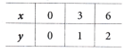
Example 2:
Draw the graph of 2x + y =6 and find the point, where graph intersects Y-axis.
Solution:
Given linear equation can be written as y = 6 -2x.
When, x = 0 then y =6 – 2(0) = 6
When, x = 1 then y = 6 – 2(1) = 6 – 2 = 4
When, x = 2 then y = 6 – 2(2) = 6 – 4 = 2
So, we have the following table to draw the graph.
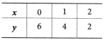
Here, we have three points A(0, 6), 5(1, 4) andC (2, 2). Now, plot these points on the graph and join them by a straight line.
Thus, we get the straight line AC, which represents the required graph of given linear equation. Also, from the graph, it is clear that the graph intersects Y-axis at the point (0, 6).
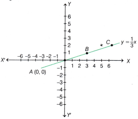
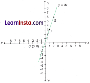
Example 3:
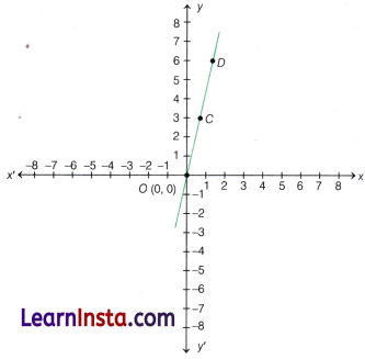
Draw the graphs of y = \(\frac{1}{3}\) x, y = x and y = 3x by selecting suitable points on these lines.
Solution:
Given linear equations are y = \(\frac{1}{2}\)x, y = x and y = 3x.
For y = \(\frac{1}{3}\)x
When, x = 0 then y = \(\frac{1}{3}\)(0) = 0
When, x = 3 then y = \(\frac{1}{3}\)(3) = 1
When, x = 6 then y = \(\frac{1}{3}\)(6)=2
So, we have the following table to draw the graph.
Here, we have three points A(0, 0), 5(3, 1) and C(6, 2).
Now, plot these points on the graph and join them by straight lines.
For y = x
When, x = 0 then y = 0
When x = 1 then y = 1
When x = 2 then y = 2
So. we have the following table to draw the graph.
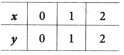
Here, we have three points 0(0, 0),D(1. I) and E(2, 2).
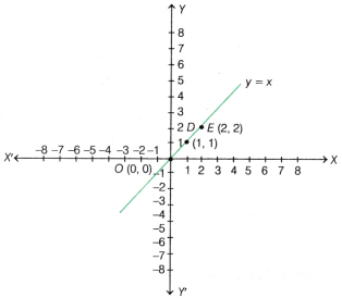
For y = 3x
When, x = 0 then y = 0
When, x = 1 then y = 3
When, x = 2 then y = 6
So, we have the following table to draw the graph.
Here, we have three points 0(0,0) F(l, 3) and G(2, 6).
Now, plot these points on the graph and join them by straight lines.
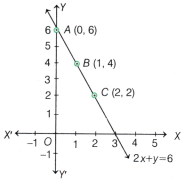
Example 4:
From the choices given below, choose the equation, whose graph is shown in the figure.
(i) x + y = 2
(ii) x – y = 2
(iii) 2x + 2y = 6
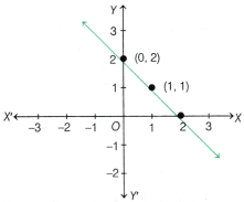
Solution:
Now, consider the equation of given graph is x + y = 2.
Given, points on the graph are (0, 2) and (1,1).
So, these points will satisfy the equation of line.
Now, at (0, 2), x + y = 0 + 2 = 2 and at (1, 1),x + y = 1 + 1 = 2
Thus, the points satisfy the equation x + y = 2.
Hence, the given graph is a graph of the equation x + y = 2.
Example 5:
If the point (2, 3) lies on the graph of the equation 2x + ay =10, find the value of a.
Solution:
Since, the point (2, 3) lies on the graph then it will satisfy its equation.
On putting x =2 and y = 3in given equation, we get 2 × 2 + a × 3 = 10
⇒ 3o = 6 ⇒ a = 2
Example 6:
Give the equation of three lines passing through (4, -5). How many more such lines are there and why?
Solution:
Clearly, the required equations are linear equations in two variables, which have solution (4, -5).
Three examples of such a linear equation are x + y = – 1, x – y = 9 and 2x + y = 3. There are infinitely many lines because there are infinitely many linear equations possible, which are satisfied by the coordinates of the point (4, -5).
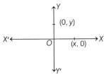
Equations of Lines Parallel to Axes
Equation of X-axis and F-axis
We know that in cartesian plane, axis XOX’ is known as X-axis and axis YOY’ is known as Y-axis.
For a point whose ordinate is zero i.e. y-coordinate is zero, we say that it is on the X-axis. So, a point of the form (a, 0) lies on X-axis.
Also, if a < 0 then it will lie on negative X-axis and if a > 0 then it will lie on positive X-axis.
Thus, equation of X-axis in one variable is y =0 and equation of X-axis in two variables is 0.x +1- y =0.
This equation shows that for each value of x, the corresponding value of y is zero i.e. the point corresponding to each solution of the linear equation lies on the X-axis.
Similarly, a point of the form (0, b) lies on Y-axis. Also, if b< 0 then it will lie on negative Y-axis and if b >0 then it will lie on positive Y-axis.
Thus, equation of Y-axis in one variable is x = 0 and equation of Y-axis in two variables is 1 . x + 0 . y = 0.
This equation shows that for each value of y, the corresponding value of x is zero i.e. the point corresponding to each solution of the linear equation lies on the Y-axis.
Equation of Lines Parallel to Y-axis
Let x – a = 0 be an equation. Then,
(i) if it is treated as an equation in one variable x only then it has a unique solution x -a, which is a point on the number line.
(ii) if it is treated as an equation in two variables x and y then it can be written as l-x+0-y-a=0. It has infinitely many solutions of the form (a, r), where r is
any real number.
Also, we can say that every point of the form (a, r) will lie on given line. Thus, given equation represents a line parallel to 7-axis.
Note:
If a > 0 then x = a represent the equation of a line parallel to Y-axis in the positive direction of X-axis and x = – a in the negative direction of X-axis.
![]()
Example 8:
Give the geometric representation of
(i) x = 4
(ii) x + 1 = 0
As an equation in one variable and in two variables.
Solution:
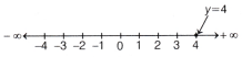
(i) Given, equation is x = 4.
When it is treated as an equation in one variable then unique solution of this equation is x = 4.
So, it is a point on number line.
![]()
When it is treated as an equation in two variables then it can be written as 1- x + 0-y = 4 and it is represented by a line.
Here, all the values of y are permissible, because 0 y is always 0.
However, x must satisfy the equation x = 4.
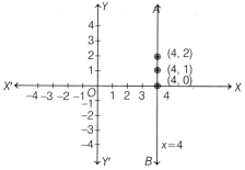
The graph AB is a line parallel to Y-axis at a distance of 4 units from Y-axis in positive direction of X-axis,
(ii) Given, equation is x + 1 = 0.
When it is treated as an equation in one variable then unique solution of this equation is x = -1.
So, it is a point on the number line.
![]()
When it is treated as an equation in two variables then it can be written as l x + 0-y + 1 = 0 and it is represented by a line.
Here, all the values ofy are permissible, because 0 y is always 0.
However, x must satisfy the equation x + 1 = 0.
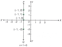
The graph PQ is a line parallel to Y-axis at a distance of 1 unit from Y-axis in the negative direction of X-axis.
Equation of Lines Parallel to X-axis
Let y – b = 0 be an equation. Then,
(i) if it is treated as an equation in one variable y only then it has a unique solution y = b, which is a point on the number line.
(ii) if it is treated as an equation in two variables x and y then it can be written as 0 – x + 1. y – b = 0. It has infinitely many solutions of the form (r, b), where r is any real number.
Also, we can say that every point of the form (r, b) will lie on this line. Thus, given equation represents a line parallel to X-axis.
Note:
If b > 0 then y = b represent the equation of a line parallel to X-axis in positive direction of Y-axis and y = -b in the negative direction of Y-axis.
Example 9:
Solve the equation 3y – 3 =13 – y and represent the solution
(i) on the number line.
(ii) in the cartesian plane.
Solution
Given equation is 3y – 3 = 13 – y
⇒ 3y + y = 13 + 3
⇒ 4y = 16
∴ y = \(\frac{16}{4}\) = 4
(i) If we treated y = 4 as an equation in one variable only then it has a unique solution y = 4.
So, it is a point on number line.
(ii) If we treated y = 4 as an equation in two variables then it can be written as 0 . x + 1 . y = 4 and it is represented by a line.
Here, all the values of x are permissible, because 0 . x is always 0.
However, y must satisfy the equation y =4.
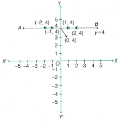
The graph AB is a line parallel to X-axis in cartesian plane at a distance of 4 units from X-axis in positive direction of Y-axis. It has infinitely many solutions as (0, 4), (1, 4), (2, 4), (3, 4), (-1,4), (-2, 4) etc.
Slope and y-intercept of a Line, Modelling Linear Growth and Linear Decay
Slope of a Linear Equation
The slope of a linear equation, representing the steepness and direction of a line. If a linear equation is written as y = mx + c
then m is the slope of the line and c is the y-intercept.
Equation of a Line in Slope-Intercept Form
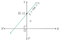
Suppose, the line L with slope m, makes an intercept c on Y-axis i.e. the line L with the slope m passes through the point (0, c). Then, the equation of the line L is given by y = mx + c
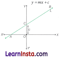
Geometrical Understanding of c
As per the equation y = mx + c, the constant c is called the y-intercept. It is the ordinate of the point, where the line intercepts the Y-axis. Also, it is the point on the line, where x = 0.
(i) If the line passes through the origin then
0 = m(0) + c ⇒ c = 0
Thus, the equation of line passing through the origin is y = mx, where m is the slope of the line.
(ii) If the line is parallel to X-axis then m = 0. Therefore, the equation of a line parallel to X-axis is y = c.
Types of Slope
- Positive slope The line rises from left to right.
- Negative slope The line falls from left to right.
- Zero slope A horizontal line.
Example 1:
Find the slope and y-intercept of the 2y – x = 4.
Solution:
Given equation is 2y – x = 4 ⇒ 2y = x + 4
⇒ y = \(\frac{1}{2}\)(x + 4)
⇒ y = \(\frac{1}{2}\)x + 2 …..(i)
On comparing Eq. (i) withy = mx + c, we get
Slope, m = \(\frac{1}{2}\) and y-intercept, c = 2
Example 2:
Find the equation of the line through (1,3) and making an intercept of 5 on the Y-axis.
Solution:
Since, y-intercept of the line, c = 5, therefore its equation is
y = mx + 5 [∵y = mx + c] …(i)
Where, m is unknown constant.
As the line (i) passes through the point (1, 3), we get 3 = m.1 + 5
⇒ m = – 2
On substituting m = -2 in Eq. (i), we get y = -2x + 5,
which is the required equation.
Example 3.
Find the slope and y-intercept of the lines \(\frac{x}{4}+\frac{y}{5}\) = 1.
Solution:
Given, equation of the line is \(\frac{x}{4}+\frac{y}{5}\) = 1.
It can be rewritten as \(\frac{y}{5}\) = 1 – \(\frac{x}{4}\)
⇒ y = \(-\frac{5 x}{4}\) + 5 …(1)
On comparing Eq. (i) with y =mx + c, we get
m = –\(\frac{5}{4}\)
and c = 5
Hence, the slope of a line is –\(\frac{5}{2}\) and y-intercept is 5.
Example 4:
Draw the graphs of the following sets of lines. In each case reflect on the role of a and b.
y = 5x, y = 3x and y = 2x
Solution:
Given, line a equations are y = 5x, y = 3x and y = 2x.
For y = 5x
When, x = 0 then y = 0
When, x = 1 then y = 5
When, x =2 then y = 10
So, we have the following table to draw the graph.
![]()
Here, we have three points 0(0, 0), A(1, 5) and B(2, 10).
Now, plot these points on the graph and join them by a straight line.

For y = 3x
When, x = 0 then y = 0
When, x = 1 then y = 3
When, x = 2 then y = 6
So, we have the following table to draw the graph.
![]()
Here, we have three points 0(0, 0), C(1, 3) and D(2, 6). Now, plot these points on the graph and join them by a straight line.
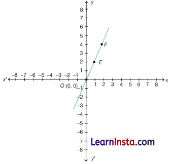
For y = 2x
When x = 0 then y = 0
When x = 1 then y = 2
When,x = 2 then y = 4
So, we have the following table to draw the graph.
Here, we have three points 0(0, 0), E(1, 2) and F(2, 4). Now, plot these points on the graph and join them by straight lines.
Modelling Linear Growth and Linear Decay
Linear models describe quantities that change by a constant amount over equal intervals of time (or another variable). Both growth and decay can be modelled using the standard linear equation.
y = mx + c
Where, y = final amount
x = independent variable (usually time or number of steps)
m = constant rate of change
and c = initial value (starting amount)
e.g. Suppose, we start a savings account with an initial deposit of ₹ 1000 and we commit to adding ₹ 200 to it every week.
So, initial amount (c) = ₹ 1000
and rate of change (m) = ₹ 200 per week
Now, polynomial expression
y = 200x + 1000
(where, y is total savings and x is the number of week.)
After 5 weeks (x = 5), the savings amount, y = 200(5) + 1000 = ₹ 2000
Example 5:
Suppose, a plant has height 2.25 feet and it grows by 0.4 feet each month.
(i) Find the height after 8 months.
(ii) Make a table of values for t varying from 0 to 10 months and show how the height h, increases every month.
(iii) Find an expression that relates h and t, and explain why it represents linear growth.
Solution:
(i) Given, initial height (c) = 2.25 feet
and rate of growth (m) = 0.4 feet per month
Now, polynomial expression
h= 0.4t + 225 …(i)
[where, h is the height and t is the number of months] After 8 months (t= 8), the height is
h = 0.4(8) + 225
= 3.2 + 2.25
= 5.45 feet
(ii) For t = 0 to 10 the values are
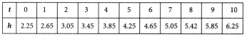
(iii) Thus, the required expression h = 0.4t + 2.25
This represents linear growth because the height increases by the same amount 0.4 feet every month.
![]()
Example 6:
A laptop is bought for ₹ 15000. Its value decreases by ₹ 1200 every year.
(i) Find the value of the laptop after 4 yr.
(ii) Make a table of values for t varying from 0 to 8 yr and show how the value of the laptop v, depreciates with time.
(iii) Find an expression that relates v and t, and explain why it represents linear decay.
Solution:
(i) Given, initial value (c) = ₹ 15,000
and rate of change (m) = – ₹ 1200 per year
Let v be the value of laptop.
Now, polynomial expression,
v = -12001 + 15000 …(i)
[where, v is the value of the laptop and t is the number of years]
After 4 yr (t = 4), the value,
v = -1200(4) + 15000 =-4800 + 15000 = 10200
(ii) For t = 0 to 8, the values are
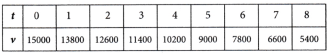
(iii) Thus, the required expression is v = -12001 + 15000.
This represents linear decay because the value decreases by the same amount 1200 every year.
Example 7:
The initial population of a town is 1200. Every year, 80 people move from a nearby city to the town.
(i) Find the population of the town after 5 yr.
(ii) Make a table of values for t varying from 0 to 10 yr and show how the population P, increases every year.
(iii) Find an expression that relates P and t, and explain why it represents linear growth.
Solution:
(i) Given, initial population (c) =1200
and rate of change (m) = 80 people per year
Let P be the population of town.
Now, polynomial expression,
P = 80t + 1200 …(i)
[where, P is the population and 1 is the number of years]
After 5 years (1 = 5) the population,
P = 80(5) + 1200 = 400 + 1200 = 1600
(ii) For t = 0 to 10, the values are
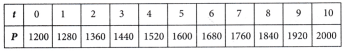
(iii) Thus, the required expression is P = 80t + 1200.
This represents linear growth because the population increases by the same number 80 people every year.